Formulation
Solid mechanics is a field that uses mathematical approaches to predict the mechanical reactions of materials to various physical conditions. To do this it does the formulation that means defining the relationship between known conditions and unknown factors of interest like stresses. To discuss how to implement the formulation, let us consider the situation depicted in the figure below.
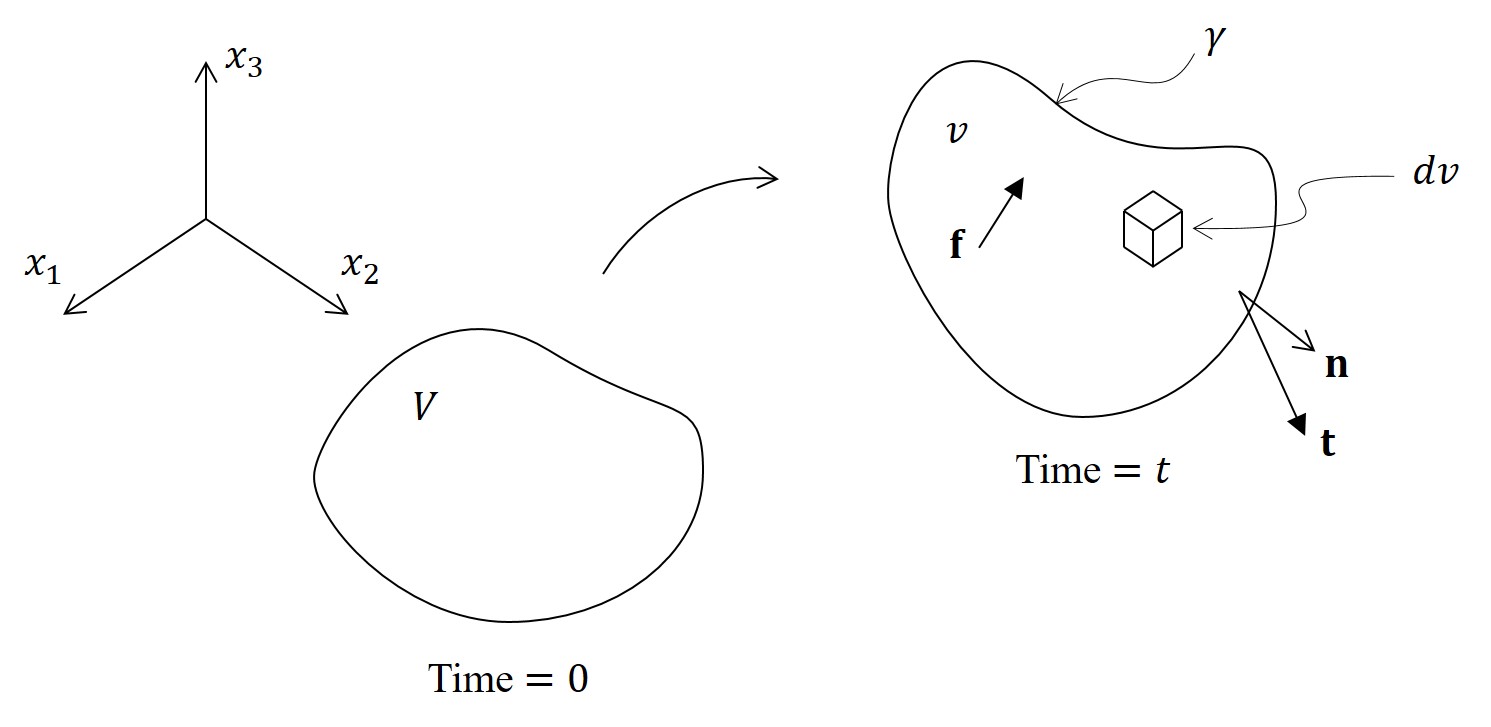
Figure 1.1 A material that deforms by body force \(\mathbf{f}\) and traction \(\mathbf{t}\).
In the figure we can see a free material that occupies volume \(V\) in the space at time \(0\), which deforms, occupying volume \(v\) at time \(t\), by body forces \(\mathbf{f}=\{f_1,f_2,f_3\}\) and surface tractions \(\mathbf{t}=\{t_1,t_2,t_3\}\), where \(f_i\) and \(t_i\) are respectively \(i\)-directional components of the body forces and the surface tractions. Note that the body forces act on volume, while surface tractions act on area. We intuitively know that, due to deformation, certain forces occur in the material body, which are called stresses. The main interest of the problems of mechanics is to calculate the stresses when the applied forces are defined. To find clues to solve the problems, we need to define the relationships between the stresses and the applied forces.
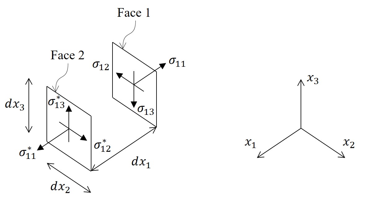
Figure 1.2 Stresses on two faces of the infinitesimal cubic volume in Figure 1.1.
Figure 1.2 shows two faces of the infinitesimal cubic volume, \(dv\) in Figure 1.1, which are parallel to the \(x_2\)-\(x_3\) plane and spaced \(dx_1\) apart from each other. On these faces stresses are acting; \(\sigma_{ij}\) on Face 1 and \(\sigma^*_{ij}\) on Face 2, where \(i=\)1 and \(j=\)1, 2, 3. Subscript \(i\) indicates the direction normal to the plane where stress is acting on, and \(j\) indicates the direction of stress. In Figure 1.2 note that the directions of \(\sigma_{1j}\) are negative \(x_j\) because the plane where they are acting on is facing in the negative \(x_1\) direction. The fact that \(dx_1\), the distance between Face 1 and Face 2 of the infinitesimal cubic volume, is very small allows us to approximate \(\sigma^*_{1j}\) by using the first order Taylor series expansion from \(\sigma_{1j}\) as
\[\sigma^*_{1j}=\sigma_{1j}+\dfrac{\partial \sigma_{1j}}{\partial x_1}dx_1=\sigma_{1j}+\sigma_{1j,1}dx_1, \tag{1.1a}\]where \(\sigma_{1j,1}\) denotes the derivative of \(\sigma_{1j}\) with respect to \(x_1\). In the same way the stresses on other planes can be written as
\[\sigma^*_{2j}=\sigma_{2j}+\dfrac{\partial \sigma_{2j}}{\partial x_2}dx_2=\sigma_{2j}+\sigma_{2j,2}dx_2, \tag{1.1b}\] \[\sigma^*_{3j}=\sigma_{3j}+\dfrac{\partial \sigma_{3j}}{\partial x_3}dx_3=\sigma_{3j}+\sigma_{3j,3}dx_3, \tag{1.1c}\]where \(\sigma^*_{2j}\) and \(\sigma^*_{3j}\) are acting on the planes facing in \(x_2\) and \(x_3\) directions, respectively.
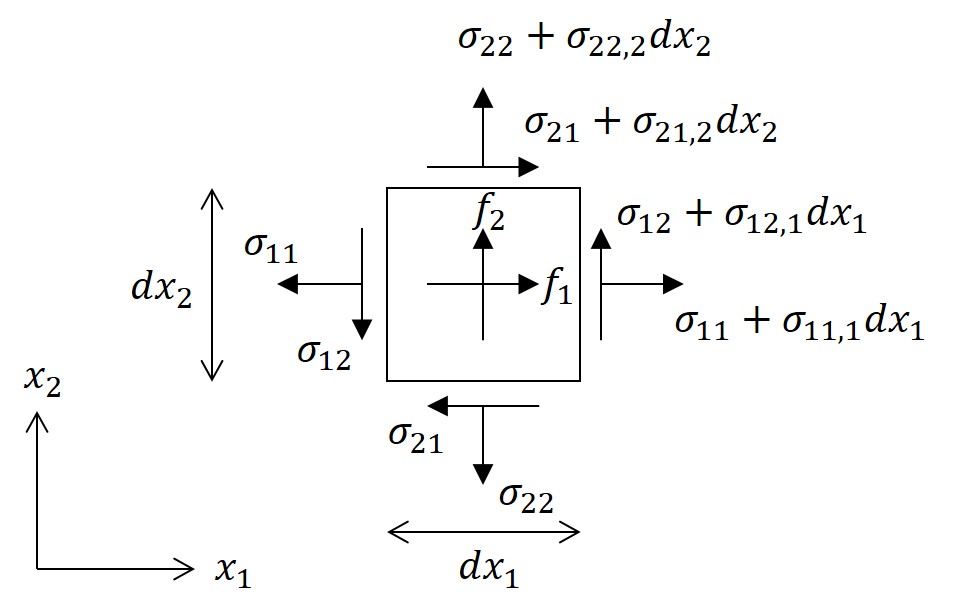
Figure 1.3 Stresses and body forces applied to the infinitesimal cubic volume viewed in the \(x_1\)-\(x_2\) plane.
Although Figure 1.3 shows the stresses and body forces applied to the infinitesimal cubic volume viewed in the \(x_1\)-\(x_2\) plane, we can imagine the situation viewed in \(x_2\)-\(x_3\) or \(x_3\)-\(x_1\) plane. If the material is in the static state, in which all forces are in equilibrium at any point, the sum of forces in each direction acting on the infinitesimal cubic volume can be written as
\[\begin{equation} \begin{aligned} \Sigma F_1 &= (-\sigma_{11}+\sigma_{11}+\sigma_{11,1}dx_1)dx_2dx_3 \\ & \ + (-\sigma_{21}+\sigma_{21}+\sigma_{21,2}dx_2)dx_1dx_3 \\ & \ + (-\sigma_{31}+\sigma_{31}+\sigma_{31,3}dx_3)dx_1dx_2 \\ & \ + f_1dx_1dx_2dx_3 \\ &= (\sigma_{11,1}+\sigma_{21,2}+\sigma_{31,3}+f_1)dx_1dx_2dx_3=0, \end{aligned} \end{equation}\tag{1.2a}\] \[\begin{equation} \begin{aligned} \Sigma F_2 &= (-\sigma_{12}+\sigma_{12}+\sigma_{12,1}dx_1)dx_2dx_3 \\ & \ + (-\sigma_{22}+\sigma_{22}+\sigma_{22,2}dx_2)dx_1dx_3 \\ & \ + (-\sigma_{32}+\sigma_{32}+\sigma_{32,3}dx_3)dx_1dx_2 \\ & \ + f_2dx_1dx_2dx_3 \\ &= (\sigma_{12,1}+\sigma_{22,2}+\sigma_{32,3}+f_2)dx_1dx_2dx_3=0, \end{aligned} \end{equation}\tag{1.2b}\] \[\begin{equation} \begin{aligned} \Sigma F_3 &= (-\sigma_{13}+\sigma_{13}+\sigma_{13,1}dx_1)dx_2dx_3 \\ & \ + (-\sigma_{23}+\sigma_{23}+\sigma_{23,2}dx_2)dx_1dx_3 \\ & \ + (-\sigma_{33}+\sigma_{33}+\sigma_{33,3}dx_3)dx_1dx_2 \\ & \ + f_3dx_1dx_2dx_3 \\ &= (\sigma_{13,1}+\sigma_{23,2}+\sigma_{33,3}+f_3)dx_1dx_2dx_3=0. \end{aligned} \end{equation}\tag{1.2c}\]Note that the areas of planes facing in \(x_1\), \(x_2\), and \(x_3\) directions are respectively \(dx_2dx_3\), \(dx_1dx_3\), and \(dx_1dx_2\). Because Equations (1.2) hold for any value of \(dx_1dx_2dx_3\) and, as explained in Stress section, \(\sigma_{ij}\) is equal to \(\sigma_{ji}\) according to the rotational equilibrium, Equation (1.2) can be expressed as
\[\sigma_{ij,j}+f_i=0; \ i,j=1,2,3,\tag{1.3}\]where, following Einstein convention, the repeated index \(j\) has the meaning of the summation, i.e., \(\sigma_{ij,j}=\sum_{j=1}^{3}\sigma_{ij,j}\). From Equation (1.3) we can see that the divergence of the stress tensor must be in balance with the body forces. The stresses must also satisfy the boundary conditions:
\[\sigma_{ij}n_j=t_i,\tag{1.4}\]where \(n_j\) is \(x_j\) directional component of \(\mathbf{n}\), a normal vector to the material surface, which is shown in Figure 1.1. Equation (1.4) means that the stresses acting on the material surface are equal to the surface tractions (see Stress section). Equations (1.3) and (1.4) are the necessary conditions that stresses must meet, which are called the governing equations. In general the governing equations are transformed into a combined solvable form by using the principle of virtual work:
\[{\delta}W=\int_v(\sigma_{ij,j}+f_i){\delta}{u_i}{dv}=0\tag{1.5},\]where \(\delta{W}\) is virtual work and \(\delta{u}_i\) is virtual displacements. The virtual displacement is a virtual candidate for deformation that may occur after time \(t\), and the virtual work is the integral of the product of the residual forces per unit volume, the left hand side of Equation (1.3), and the virtual displacements. Because the residual forces per unit volume vanish in equilibrium, as can be seen in Equation (1.3), the virtual work inevitably has a value of zero. In Equation (1.5) note that the summation is taken over the repeated subscripts \(i\) and \(j\), therefore, the virtual work is a scalar. Using the property of differentiation below,
\[(\sigma_{ij}\delta{u_i})_{,j}=\sigma_{ij,j}\delta{u_i}+\sigma_{ij}\delta{u_{i,j}},\tag{1.6}\]Equation (1.5) can be written as
\[\int_v(\sigma_{ij}\delta{u_i})_{,j}{dv}-\int_v\sigma_{ij}\delta{u_{i,j}}{dv}+\int_v{f_i}{\delta}{u_i}{dv}=0\tag{1.7}.\]By noting that \((\sigma_{ij}\delta{u_i})_{,j}\) implies the divergence of \(\sigma_{ij}\delta{u_i}\) and applying the divergence theorem to its integral over the volume, we can rewrite Equation (1.7) as
\[\int_\gamma\sigma_{ij}n_j\delta{u_i}{da}-\int_v\sigma_{ij}\delta{u_{i,j}}{dv}+\int_v{f_i}{\delta}{u_i}{dv}=0\tag{1.8},\]where \(\int_\gamma{da}\) is the area integral over the material surface \(\gamma\). Substituting Equation (1.4) into (1.8) gives
\[\int_v\sigma_{ij}\delta{\varepsilon_{ij}}{dv}-\int_v{f_i}{\delta}{u_i}{dv}-\int_\gamma{t_i}\delta{u_i}{da}=0\tag{1.9},\]where \(\delta{u_{i,j}}\) in Equation (1.8) is replaced to \(\delta\varepsilon_{ij}=\frac{1}{2}(\delta{u_{i,j}}+\delta{u_{j,i}})\), the symmetric part of \(\delta{u_{i,j}}\), by taking into account the symmetry of \(\sigma_{ij}\). Equation (1.9) is called the weak form for the governing equations.
In many cases, the use of the weak form is preferable to that of the strong form for some reasons. Firstly the weak form contains the equilibriums for body forces and surface tractions, represented in Equations (1.3) and (1.4), in a single equation. It is also compatible with the energy equations which are useful when considering specific physical conditions, such as contact or incompressibility. Additionally, the weak form is more suitable when implementing the finite element analysis which is one of the most widely used approaches to solve modern mechanics problems.